
When people hear the phrase “Artificial Intelligence(AI)”, they often imagine some complicated self-aware robot from sci-fi movies. However, AI actually has a very general definition of “Machines that can perform tasks that normally requires human intelligence”. With this definition, anything from self-driving cars to the “line of best fit” feature in Excel can be considered AI.
Gradient descent is a simple, intuitive, and very useful and effective approach to data modeling and is categorized under a branch of AI called machine learning(ML). Gradient descent is often used to find line of best when given multiple data points. There are three basic component to running a gradient descent algorithm: the training examples, the parameter, and the cost function. The training examples refer to data that is used to “train” the gradient descent algorithm. For example, if the goal of a gradient descent algorithm is to predict house prices based on size, the training examples will be a list of sizes of existing houses and their respective price. The parameter, often referred as theta(θ), is the coefficients of the function that the algorithm uses to model the data. For example, if the line of best fit is in the format of f(x) = ax2+bx+c, a, b, and c will be the parameters. The cost function, or J(θ), is a representation of how well can the data be modeled with respect to different parameters. The lower the cost, the better the fit of the function to the training examples.
Gradient descent works in four steps. First, it starts with a set of random θ values. Second, it calculates the gradient of the cost function with respect to the current θ. Third, it modifies θ by subtracting the gradient of the cost function from θ using the equation θ = θ – α*J’(θ)). The α(alpha) in the equation is just a coefficient called “learning rate” used to determine how fast the algorithm will run. Forth, it repeats the second and third step until the cost is at the current θ is at the local or global minimum of J(θ).
Gradient descent works because of the concavity of cost functions. When the cost function is graphed with respect to θ, it will look something like this:
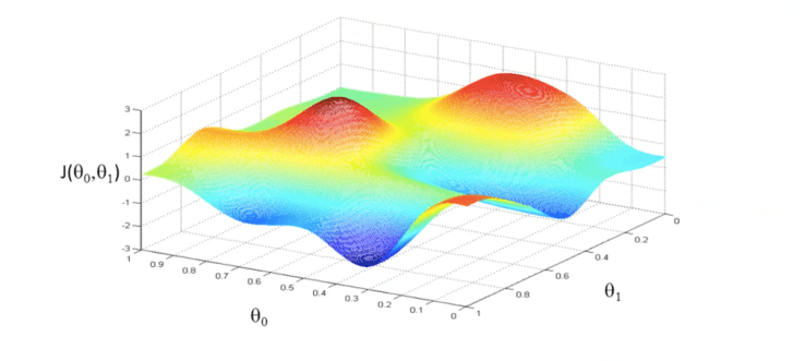
A Cost Function Graphed With Respect to θ
What gradient descent does is like dropping a ball down a random point on the curve made by the cost function. Naturally, the ball will “roll” to the lowest point of the cost function, giving the algorithm the θ that will minimize the cost function. The learning rate acts like the gravity setting and determines how fast the ball rolls.
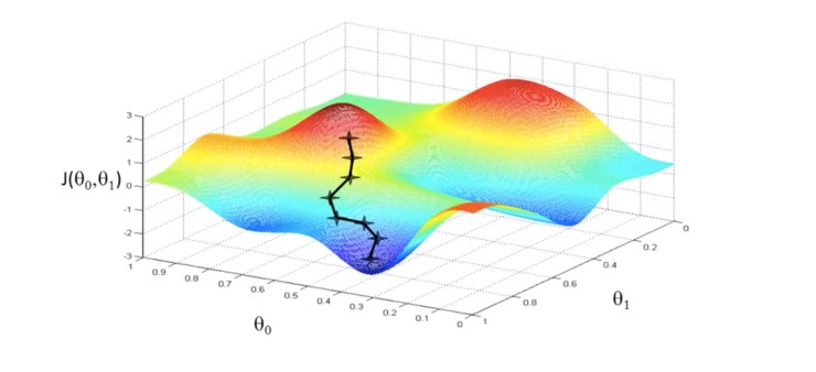
Gradient Descent Doing Its Magic
Gradient descent sometimes end up in local but not global minimums, especially when there’s a lot of parameters in θ, but it is still one of the most commonly used machine learning algorithm due to its ease to implement and reliable results.
Bibliography
“Machine Learning” Coursera, Stanford University, http://www.coursera.org/learn/machine-learning/home/welcome.